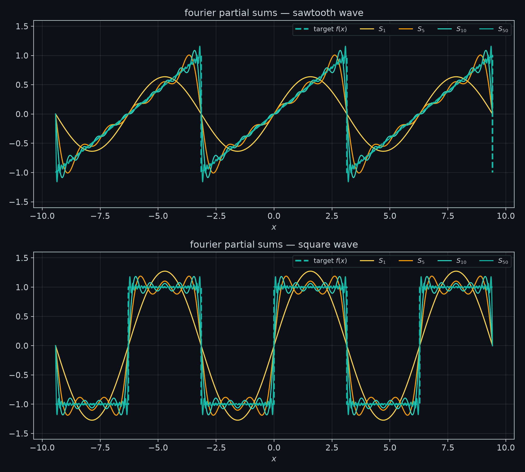
Take a periodic signal — any periodic signal, even one with sharp jumps — and you can rebuild it out of nothing but sines and cosines. That claim, which Joseph Fourier made in 1807 while studying how heat flows through solids, scandalized the mathematicians of his time. This experiment makes the claim visible: we reconstruct two classic waveforms term by term, watch the reconstruction sharpen as terms accumulate, and meet the one place where the promise breaks down in a beautiful way.

Everything below was computed with NumPy and Matplotlib (Python 3.14, NumPy 2.5); the code snippets are the actual pieces doing the work.

the setup #

For a $2\pi$-periodic function $f(x)$, the Fourier series is

with coefficients obtained by projecting $f$ onto each basis function:

The projection works because the trigonometric family is orthogonal on $[-\pi, \pi]$: the integral of $\sin(nx)\sin(mx)$ vanishes unless $n = m$. (The experiment checks this numerically — the largest off-diagonal inner product comes out at $5.6 \times 10^{-17}$, machine noise.)

Symmetry does half the work for us. Both functions below are odd, $f(-x) = -f(x)$, so every cosine coefficient $a_n$ vanishes and we are left with pure sine series.

case study 1 — the sawtooth wave #

The sawtooth is the linear ramp $f(x) = x/\pi$ on $(-\pi, \pi)$, repeated forever. Integration by parts on the projection integral gives

so the series is

Every harmonic contributes, and the amplitudes fall off slowly, like $1/n$ — a signature of the jump discontinuity at the edges of each period.

case study 2 — the square wave #

The square wave alternates between $+1$ on $(0, \pi)$ and $-1$ on $(-\pi, 0)$. Splitting the projection integral at the jump:

Only odd harmonics survive — the square wave's half-wave symmetry silences every even one:

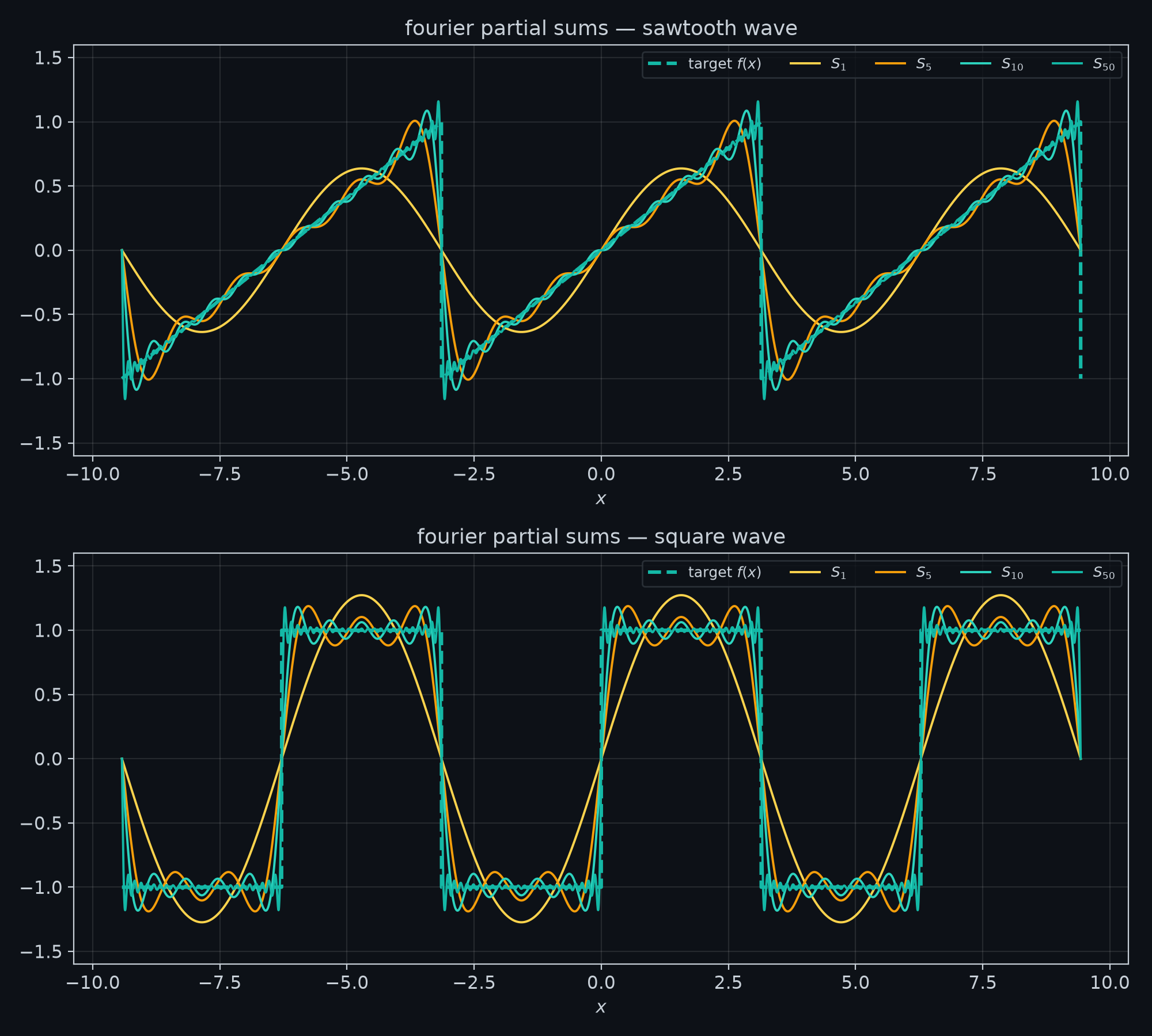
Computing the partial sums $S_N$ for both waves is three lines of vectorized NumPy — build all terms at once, then let a cumulative sum produce every truncation level simultaneously:

n = np.arange(1, N_MAX + 1)
terms = coeffs[:, None] * np.sin(n[:, None] * x[None, :])
partial_sums = np.cumsum(terms, axis=0)   # row N-1 holds S_N(x)

watching the series converge #

Static overlays compress the story; the animation tells it properly. Here is the reconstruction sharpening as $N$ climbs from 1 to 100:

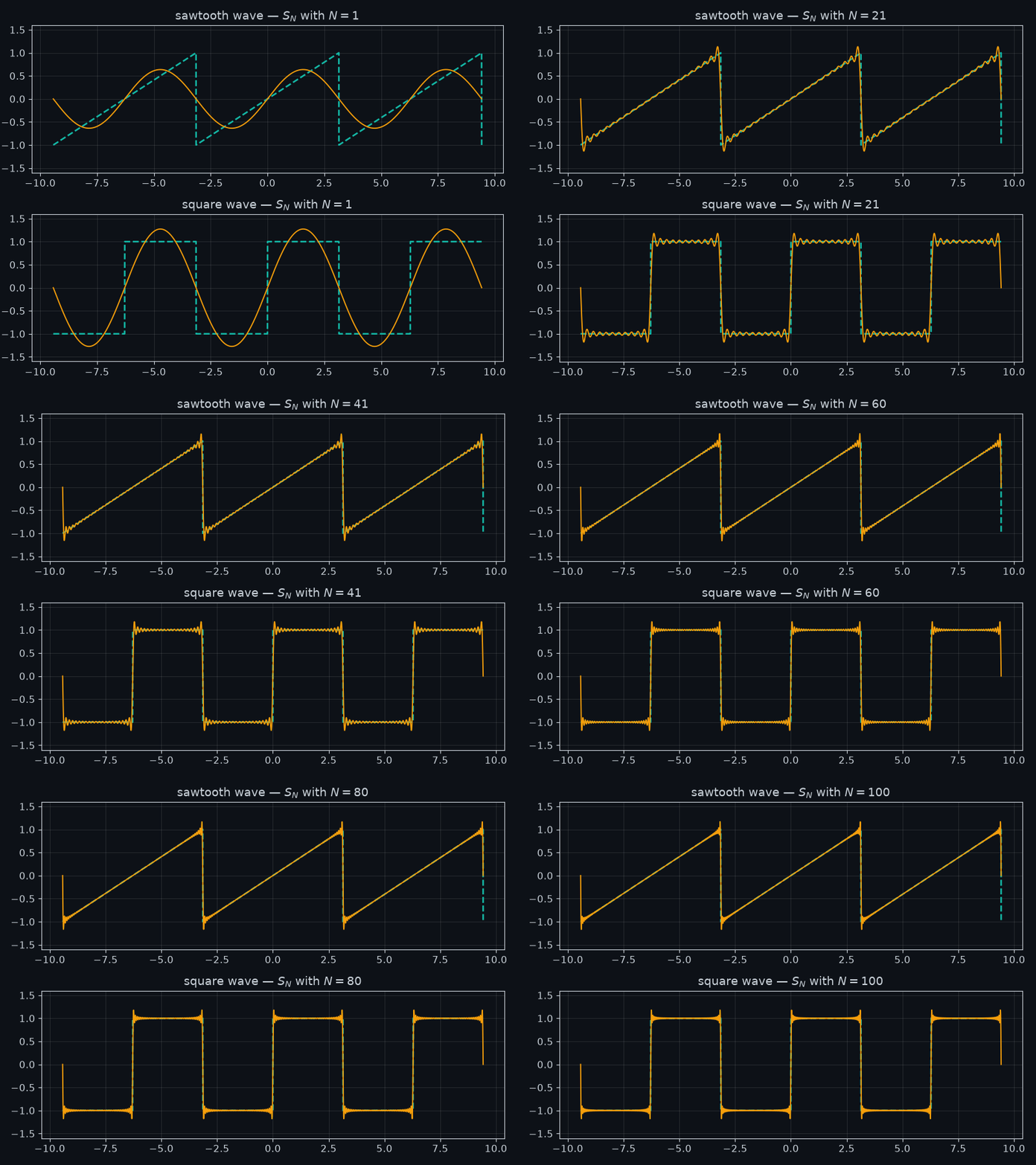
Two behaviors are worth separating. Away from the jumps, the error melts away steadily and the approximation hugs the target. At the jumps, the wiggles compress horizontally but their peak height stops shrinking. That refusal has a name.

the gibbs phenomenon #

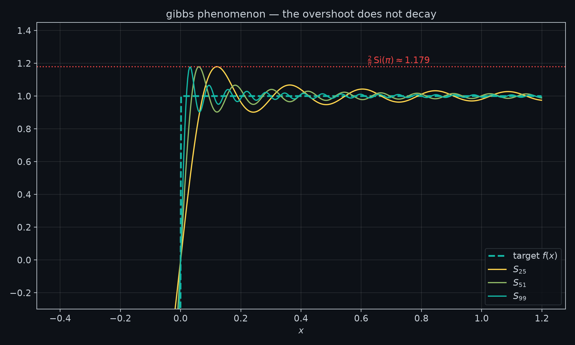
The experiment measures the peak of $S_{100}$ at $1.1790$, matching the theoretical constant to four decimal places. This is not a numerical artifact: it is the price of building a discontinuous function out of continuous pieces, and it is why naive truncation is a poor low-pass filter for signals with sharp edges.

how fast is convergence? #

Parseval's identity connects the coefficients to the signal's energy: the integral of $f^2$ over one period equals $\pi \sum b_n^2$. (Numerically the identity holds to within 0.6% at $N = 100$ — exactly the energy left in the truncated tail.) It also predicts the convergence rate. The squared $L^2$ error of $S_N$ is the tail energy

since $b_n \sim 1/n$ for both waves.

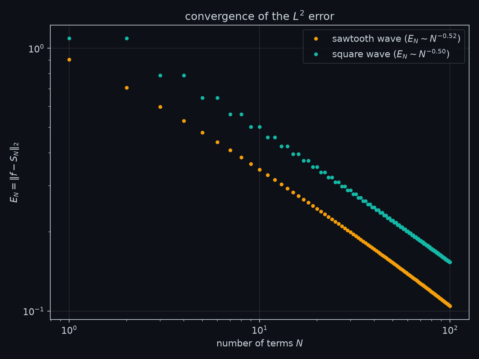
The fitted slopes land on $-0.52$ and $-0.50$. That slow square-root decay is entirely the fault of the jumps; make the function continuous (a triangle wave, say) and the coefficients fall like $1/n^2$, buying a full extra order of convergence.

what the experiment validated #

Every figure above sits on top of assertions that ran before any plotting: the numerically integrated coefficients match the derived formulas to a relative error below $5 \times 10^{-7}$, the sine basis is orthogonal to machine precision, Parseval's identity balances to under 1%, and the Gibbs peak reproduces $\frac{2}{\pi}\operatorname{Si}(\pi)$. Validation before visualization — otherwise a pretty animation can hide a wrong sign for a long time.

takeaways #

Fourier series really do rebuild arbitrary periodic signals from pure tones — with two honest footnotes. Convergence is only as fast as the function is smooth, and discontinuities exact a permanent 9% toll at the jump. Both footnotes are visible to the naked eye once you animate the partial sums, which is the whole point of doing this computationally.

Next in this series: the same convergence questions asked of Taylor polynomials, where the failure mode is not an overshoot but a hard wall — the radius of convergence.